KNN

These are the nights that never die!

Introduction to K-Nearest Neighbors Classifier

KNN is a very easy algorithm.

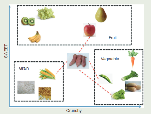
kNN classifier is to classify unlabeled observations by assigning them to the class of the most similar labeled examples. Characteristics of observations are collected for both training and test dataset. For example, fruit, vegetable and grain can be distinguished by their crunchiness and sweetness.

There are two important concepts in the above example.

1.Distance

Minkowski Distance

In fact, it`s not a sort of distance, but a defination of distance.

$$d_{xy} = \sqrt[q]{\sum_{k=1}^{n}(x_k-y_k)^p}$$

where p is a variable parameter

if p = 1 Manhattan Distance

$$D = \sum_{k=1}^{n}{|x_k-y_k|}$$

if p = 2 Euclidean Distance

if p = Chebyshev Distance

$$D = max|x_i-y_i|,1\leq i \leq n$$

Euclidean distance

By default, the knn() function employs Euclidean distance which can be calculated with the following equation

$$D(p,q) = \sqrt{(p_1-q_1)^2+(p_2-q_2)^2+......+(p_n-q_n)^2}$$

where p and q are subjects to be compared with n characteristics.

2. Parameter K

The appropriate choice of k has significant impact on the diagnostic performance of kNN algorithm.

The key to choose an appropriate k value is to strike a balance between overfitting and underfitting.

Some authors suggest to set k equal to the square root of the number of observations in the training dataset.

Let’s talk about the differences between approximate error(近似误差) and estimation error(估计误差):

approximate error: a taining error for training set

只能体现对训练数据的拟合表现。

estimation error: a testing error for testing set

可体现对测试数据的拟合表现，也就是体现出泛化能力，因此对模型要求是估计误差越小越好。

In practical applications , we usually choose a pretty smaller parameter k which aims to get the best parameter k.

Implementation

from sklearn.datasets import load_iris
from sklearn.model_selection import train_test_split
from sklearn.preprocessing import StandardScaler
from sklearn.neighbors import KNeighborsClassifier

def knn_iris():
    #1.获取数据集
    iris = load_iris()
    #2.划分数据集
    x_train ,x_test , y_train , y_test =  train_test_split(iris.data,iris.target,random_state=6)
    #3.特征工程
    transfer = StandardScaler()
    x_train = transfer.fit_transform(x_train)
    #这里就是说测试集要用训练集的平均值和标准差
    #如果在之前统一标准化的话，训练集和测试集的数据成分就混了
    #如果test也用fit，则test用了自己的计算，就不再与train一致了
    x_test = transfer.transform(x_test)
    #4.KNN
    estimator = KNeighborsClassifier(n_neighbors=3)
    estimator.fit(x_train,y_train)
    #5.模型评估
    #法1.比对真实值和预测值
    y_predict = estimator.predict(x_test)
    print("y_predict:\n",y_predict)
    print("直接对比真实值和预测值:\n",y_test == y_predict)
    #法2.计算准确率
    score = estimator.score(x_test,y_test)
    print(score)

if __name__ == "__main__":
    knn_iris()

Evaluations

Advantages

①High accuracy(高精度)

②Insensitive to outliers(对异常值不敏感)

③No data entry assumes(无数据输入假定)

Disadvantages

High computational complexity and high spatial complexity (计算复杂度高、空间复杂度高)

Differences Between Regression and Classification

	Regression	Classification
Output	Quantitative(定量)	Qualitative(定性)

KNN Regression

$$\hat{y} = \frac{1}{K} \sum_{i=1}^{K}y_i$$

Data normalization(数据归一化处理)

使用零均值归一化：

$$z = \frac{x-\mu}{\sigma}$$

Code

import numpy as np
import matplotlib.pyplot as plt
from sklearn.preprocessing import StandardScaler
from sklearn.neighbors import KNeighborsRegressor

transformer = StandardScaler() #数据预处理归一化
x_train = np.array([
    [158, 1],
    [170, 1],
    [183, 1],
    [191, 1],
    [155, 0],
    [163, 0],
    [180, 0],
    [158, 0],
    [170, 0]
])
x_train_scaled = transformer.fit_transform(x_train)
y_train = [64, 86, 84, 80, 49, 59, 67, 54, 67]

x_test = np.array([[168, 1],
    [180, 1],
    [160, 0],
    [169, 0]])
x_test_scaled = transformer.transform(x_test)
y_test = [65, 96, 52, 67]
##=============================上面是导入数据
K = 3
clf = KNeighborsRegressor(n_neighbors=K)
clf.fit(x_train_scaled,y_train)
predictions = clf.predict(np.array(x_test_scaled))
print('Predicted weights: %s' % predictions)
print('Actual weights: %s' % y_test)
print('========回归评估:=======')

from sklearn.metrics import mean_squared_error 
from sklearn.metrics import mean_absolute_error
from sklearn.metrics import r2_score

print('决定系数: %.4f' % r2_score(y_test, predictions))
print('均方差: %.4f' % mean_squared_error(y_test, predictions))
print('平均绝对误差: %.4f' % mean_absolute_error(y_test, predictions))